II: Theoretical foundations

Recall from the first chapter that our focus is going to be a task called “datamodeling” or “predictive data attribution,” where our goal is to predict how models will behave when trained on different training datasets. It turns out that in classical statistics, this problem has been studied extensively. Predicting such data counterfactuals is of significant interest in, for example, cross-validation, the bootstrap, etc.

Why “predictive data attribution”/“datamodeling”? The problem of predicting model changes as a function of training dataset changes is an age-old problem, especially in statistics: names like “influence functions” (Hampel 1974), “von Mises calculus” (von Mises 1947), “regression analysis” (Pregibon 1981), and “infinitesimal jackknife” (Jaeckel 1972), all refer to this problem (or variants thereof, or methods for solving it). We use the names “predictive data attribution” or “datamodeling” as a catchall for all of these terms, emphasizing the connection to data attribution.

Help us find references! Nothing here is new—this chapter surveys and draws from an extensive line of work in statistics and beyond. In particular, the literature on predicting data counterfactuals is incredibly broad and we’ve surely missed some references or incorrectly attributed techniques. If you think this is the case, please let us know! ml-data-tutorial@mit.edu

Notation, Definitions, and Problem Setup

Before we get into it, we’ll introduce some definitions and notation that will come in handy throughout the rest of this chapter.

Notation. Let’s start with some notation—we’ll try to explicitly recall these when we use them. Throughout this chapter, we will use lowercase for scalars $a \in \mathbb{R}$, bold for vectors $\bm{v} \in \mathbb{R}^n$, and uppercase for matrices $M \in \mathbb{R}^{n \times m}$.

We’ll use $\bm{1}_n$ to represent the $n$ dimensional all-ones vector, and $\text{Ind}_n[j]$ to represent a “one-hot” vector of dimension $n$ that is equal to $1$ at index $j$ and $0$ everywhere else.

For a differentiable function $f: \mathbb{R}^n \to \mathbb{R}$ mapping vectors to scalars, we will use $\nabla f(\bm{v}) \in \mathbb{R}^n$ to denote the gradient of $f$ with respect to its argument, and similarly $\nabla^2 f(\bm{v})$ the Hessian of $f$ with respect to its argument. For a vector-valued function $f: \mathbb{R}^n \to \mathbb{R}^m$, we will use $\mathbf{J}_{\bm{v}}[f] \in \mathbb{R}^{n \times m}$ to denote the Jacobian of $f$ evaluated at $\bm{v}$.

Our focus: (Weighted) loss minimization. In this chapter, our focus will be on estimating parameters $\theta^\ast$ that minimize an average of loss functions. That is, for some collection of loss functions $\lbrace \ell_1, \ell_2,\ldots,\ell_n \rbrace$,

For example, we can think of the $\theta^\ast$ as parameters of a machine learning model, where $\ell_i(\theta)$ represents the loss of a model with parameters $\theta$ on the $i$-th example in the training dataset.

Note: In statistics, parameters $\theta$ of this form (i.e., parameters that minimize a sample average of losses) are called M-estimators.

In order to instantiate a very general version of the counterfactual prediction problem, we’re going to extend the definition above to capture a weighted collection of loss functions. In particular, we’ll consider a weighting $\bm{w} \in \mathbb{R}^d$, and define $\theta^\ast(\bm{w})$ as:

Leave-one-out score. We can use the notation we’ve defined so far to set up the most basic version of a data counterfactual: the leave-one-out (LOO) counterfactual. This is simply the counterfactual effect of leaving out one loss function $\ell_j$, i.e.,

Note that using the notation we’ve introduced, we can rewrite the LOO score as:

Since much of this chapter is going to focus on the leave-one-out score, we’ll also introduce some shorthand for the two parameter vectors above, letting

allowing us to rewrite the leave-one-out counterfactual as

Warm-up: Leave-one-out estimation for OLS

As a warm-up exercise, let’s think about a simple linear regression. Here we have a set of covariates $\lbrace \bm{x_1},\ldots,\bm{x_n}: \bm{x_i} \in \mathbb{R}^{d}\rbrace$, and corresponding outcomes $\lbrace y_1,\ldots y_n: y_i \in \mathbb{R}\rbrace$. Our goal is to find a linear parameter $\theta^\ast$ that best predicts $y$ as a function of $\bm{x}$—in keeping with the rest of this section, we’ll further parameterize the problem with a set of data weights $\bm{w} \in \mathbb{R}_{+}^{n}$:

Now, this minimization problem has a rather well-known closed-form solution:

Using this closed form, we can actually derive a closed form for the leave-one-out score $LOO(j)$. In particular, observe that

We can simplify this expression considerably using the Sherman-Morrison formula, given below:

Applying the formula (and a bit of algebra), we arrive at:

and so, letting $M = \sum_{i=1}^n \bm{x_i}\bm{x_i}^\top$ be the empirical covariance matrix of the data, we have that

Although slightly long, the form above is actually both conceptually simple and easy to compute. The ${\color{blue} \text{blue}}$ term is simple the residual of a model trained on the full dataset evaluated on the left-out point $\bm{x_j}$, and the ${\color{darkred} \text{denominator}}$ is a relatively common quantity known as the leverage score of the point $\bm{x_j}$. The main cost in computing the above is calculating $M^{-1}$, but we actually get this for free, since $M^{-1}$ goes into $\theta^\ast$.

Leave-one-out for more complicated (linear) models

So, it turned out that leave-one-out scores have a convenient closed form when it comes to linear regression, that relied only on computing the initial parameters $\theta^\ast$ and then computing matrix-vector products on the sample $(\bm{x_j}, y_j)$ whose leave-one-out effect we want to quantify.

Unfortunately, to get this closed form, we relied pretty heavily on the existence of a closed-form solution to the least-squares problem itself. When we get to even slightly more complicated models like logistic regression (which is still linear but has no closed form), things become quite complicated. For now, let’s assume that we are dealing with a linear model, i.e.,

where recall that $\lbrace \bm{x_1},\ldots,\bm{x_n}\rbrace$ are our inputs.

Our running example will be a 2D logistic regression problem, where $\bm{x_i} \in \mathbb{R}^2$, $y_i \in \lbrace -1, 1\rbrace$ and $L_i(\mu) := \sigma(y_i \cdot \mu)$:

Solving for parameters $\theta^\ast(w)$ here entails running an iterative algorithm like gradient descent to minimize the loss. How do we compute the leave-one-out score in the absence of a closed form?

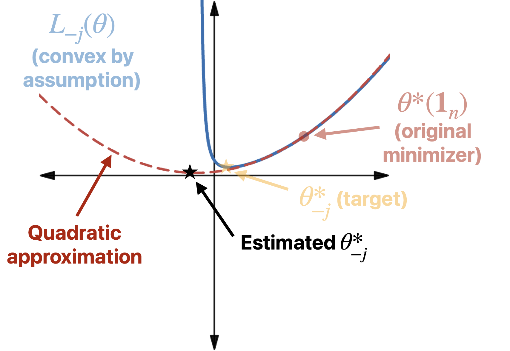
One clever idea is to leverage Newton’s method (this was suggested as early as Pregibon (1981), but studied a lot in the 21st century too). The key realization is that $\theta^\ast_{-j}$ is the minimizer of the function

Starting from $\theta^\ast = \theta^\ast(\bm{1}_{n})$ (which, remember, is the optimal parameter vector for the unweighted loss), we can quadratically approximate $L_{-j}(\theta)$, i.e.,

and then minimize this quadratic approximation with respect to $\bm{\delta}$ to obtain our estimate for $\theta^\ast_{-j}$.

where $L’$ and $L’’$ are the first and second derivatives of $L$, respectively. Using the exact same technique (the Sherman-Morrison formula) as for linear regression, and using the fact that, by definition of ${\theta^\ast}$ as the optimal parameter, $\sum_{i=1}^n L_i’({\theta^\ast}^\top \bm{x_i}) \cdot \bm{x_i} = 0$, we get the following LOO estimator.

Conceptually, our estimator looks something like this:

How well does this work? Let’s return to our running example of logistic regression. There, $L_i({\theta^\ast}^\top \bm{x_i}) = \sigma(y_i \cdot {\theta^\ast}^\top \bm{x_i})$ (where $\sigma(\cdot)$ is the sigmoid function), and so

Plugging these in yields the following estimate for the leave-one-out counterfactual:

def newton_estimate_loo(orig_model, X, y, j):
  ps = orig_model.predict_proba(X) 
  correct_ps = [np.arange(N_SAMPLES), y]
  M = np.linalg.inv(X.T @ np.diag(ps[:,0] * (1 - ps[:,0])) @ X)
  y = 2 * y - 1 # Translate {0, 1} -> {-1, 1}
  p_j = correct_ps[j]
  
  num = M @ X[j] * (1 - p_j) * y[j] # Mx * L'
  denom = 1 - X[j] @ M @ X[j] * (1 - p_j) * p_j # 1 - x^T M x * L''
  return num / denom

Furthermore, under some assumptions (e.g., if the covariates $\bm{x}_i \in \mathbb{R}^d$ are drawn from a $d$ dimensional Gaussian distribution, and if the loss functions $L_i$ are strongly convex and have smooth enough derivatives), Rad and Maleki (2020) show that the estimate above for $LOO$ perfectly predicts out-of-sample error (i.e., the loss on $\bm{x}_j$) as $n, d \to \infty$ (with $n / d = \delta_0$).

Comparing to linear regression. In the case of least squares, $L_i(\hat{y}) = \frac{1}{2}(\hat{y} - y_i)^2$, and so $L_i’(\hat{y}) = (\hat{y} - y_i)$ and $L_i’’(\hat{y}) = 1$. Plugging these in to the estimator above yields

In other words, we recover exactly the closed-form solution! (This isn’t really a coincidence: our estimator used a quadratic approximation of the loss, which is actually exact for OLS.)

What about non-linear models? And leave-k-out?

In the last section, we saw how Newton’s method yields a reasonable approximation to leave-one-out scores for linear models without closed-form solutions. Recall that our original goal, however, was not just to predict leave-one-out scores: we want to be able to predict how arbitrary changes to the dataset are going to change models. And we also don’t want to limit ourselves to models that are linear in the covariates.

One natural idea would be to use the same Newton step approach as last time—unfortunately, we immediately find that many of the simplifications don’t work. Instead, we’re going to use another clever (and very old) idea: Taylor approximation! Rather than try to estimate the effect of dropping out data points, we’ll try to estimate the effect of infinitesimally up- or down-weighting them, and then use those estimated infinitesimal effects to extrapolate to large changes in the datasetThis technique is commonly referred to as the infinitesimal jackknife, or the influence function. . Mathematically, we are going to approximate:

where $\mathbf{J}_{\bm{w} = \bm{1}_n}[\theta^\ast(\bm{w})]$ is the Jacobian matrix, with entries

This expression actually works as an approximation to $\theta^\ast(\bm{w})$ for any $\bm{w}$, and is not limited to LOO approximations. To actually go about computing it, though, we need to find the Jacobian $\mathbf{J}$. We’ll do this by leveraging the fact the fact that

\(\theta^\ast(\bm{w}) = \arg\min_\theta \sum_{i=1}^n w_i \cdot \ell_i(\theta),\) and so first-order optimality conditions tell us that \(\sum_{i=1}^n w_i \cdot \nabla_\theta \ell_i(\theta^\ast(\bm{w})) = 0.\) Differentiating both sides with respect to $w_i$,

Finally, re-arranging gives:

The Jacobian $\mathbf{J}$ is given by stacking the rows $\frac{d\theta^\ast(w)}{dw_i}$: plugging this into the Taylor estimator above, we get the following estimator:

How does this relate to our Newton-based estimator above? Mathematically, if we instantiate the estimator above in the context of logistic regression, we get

In particular, we get the same exact expression as what we got from the quadratic approximation, with the exception that we now omit the denominator $1 - \bm{x_j}^\top M \bm{x_j}\cdot \mathcal{L}’’({\bm{\theta^*}}^\top \bm{x_j})$. One implication of this is that even for least-squares linear regression, our new estimator no longer exactly recovers $LOO(j)$ as given by the closed form expression. Nevertheless, the resulting estimator is extremely general—we can now move beyond linear problems—and still works pretty well:

Perhaps more convincingly than the single logistic regression example above, Giordano et al. give fairly general conditions under which one can get finite-sample guarantees on the performance of this estimator.

Takeaways

In this section, we studied a close statistical analog of the predictive data attribution/datamodeling problem from statistics, where the goal is to estimate how the minimizer of a sum of strongly convex loss functions changes as a function of the weights placed on each loss function. In the case of ordinary least squares, the problem turned out to have an exact closed form. For slightly more complicated (but still linear) problems, we used a quadratic approximation to the loss function in order to derive an approximate estimator called the Newton Step estimator. Finally we used a Taylor approximation—estimating the effect of infinitesimally upweighting or downweighting points—in order to come up with a general estimator for non-linear (but still strongly convex) problems.

In the next section, we’re going to shift our focus to the study of the (much messier) deep learning landscape—will the same tools prevail, or will we need new techniques?

Some links and resources

Below is an incomplete list of resources that talk more about the theory of predictive data attribution:

1. Daryl Pregibon. Logistic Regression Diagnostics (1981)
2. Kamiar Rahnama Rad, Arian Maleki. A scalable estimate of the extra-sample prediction error via approximate leave-one-out (2020)
3. Ryan Giordano, Will Stephenson, Runjing Liu, Michael I. Jordan, Tamara Broderick. A Swiss Army Infinitesimal Jackknife (2020)
4. Frank Hampel. The Influence Curve and its Role in Robust Estimation (1974)
5. Jun Shao, Dongsheng Tu. The Jackknife and Bootstrap (1995)