
IV: Data attribution in the wild
In the final part of this tutorial, we overview applications of (predictive) data attribution—both mature and up-and-coming—in large-scale settings. We’ll cover four topics:
As a roadmap: we cover these applications in two separate parts below. First, we briefly describe model debugging, which is an application of all categories of data attribution methods. We then cover the latter three applications (data selection, machine unlearning, and data poisoning) in a common predictive data attribution-based framework.
Model debugging
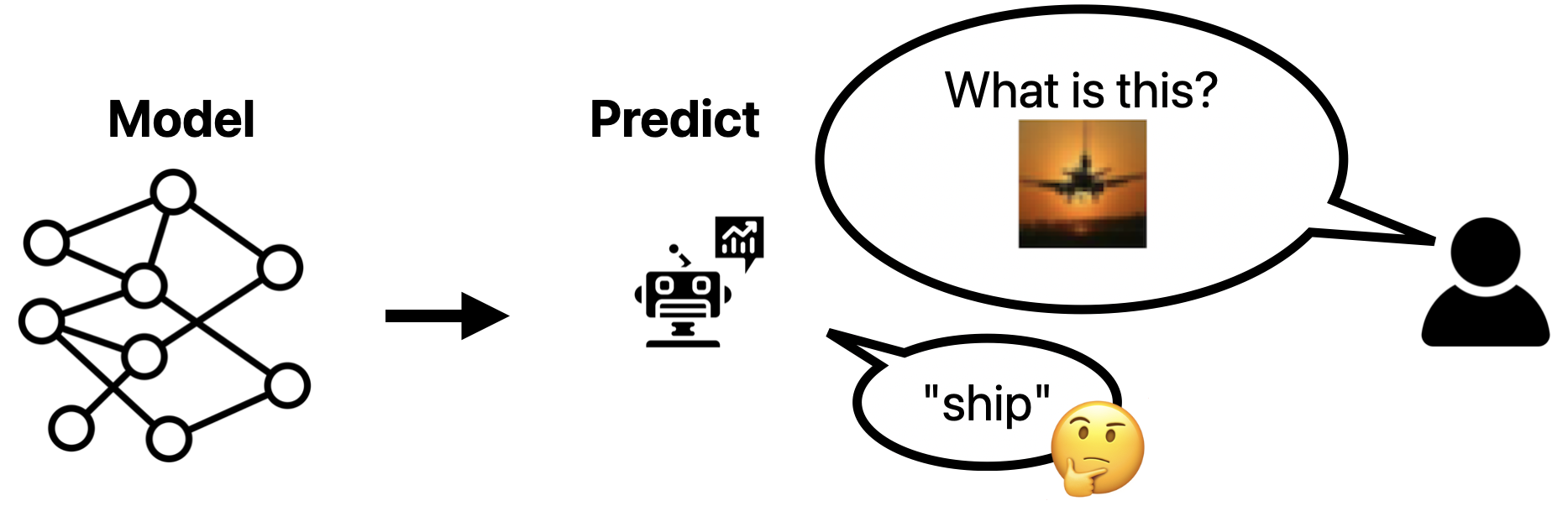
We often want to understand why models behave the way they do. For example, we may want to understand why a classifier incorrectly predicts:
Data attribution methods do not directly explain why a model made the predictions it did. However, such methods do help in a crucial step of the understanding process: generating potential hypotheses that could explain the observed behavior.
A data-centric view of model behavior. Methods for generating hypotheses that might explain model behavior range from tracing model weights to correlating human interpretable concepts with model outputs. In this section, we turn to the dataset to identify possible hypotheses; after all, the training dataset (in large part) determines trained model behavior. Unfortunately, it is hard to surface potential mechanisms for model behavior by simply inspecting the training dataset directly. Training sets are generally too large for humans to “understand” in a meaningful way. Furthermore, simply inspecting training data samples may not necessarily yield insights on model behavior, as models learn unintuitive features from data. To make analyzing the dataset more tractable, one solution is data attribution.
Debugging with data attribution. Consider the scenario above, where we aim to understand why a CIFAR-10 model corrected incorrectly on a photo of a plane on a sunset. A common data attribution-based approach for identifying potential explanations is to assign each training sample an importance, then inspect the “high importance” samples. For example, a predictive data attribution method, surfaces the following “most important” training samples for the test sample of interest above:
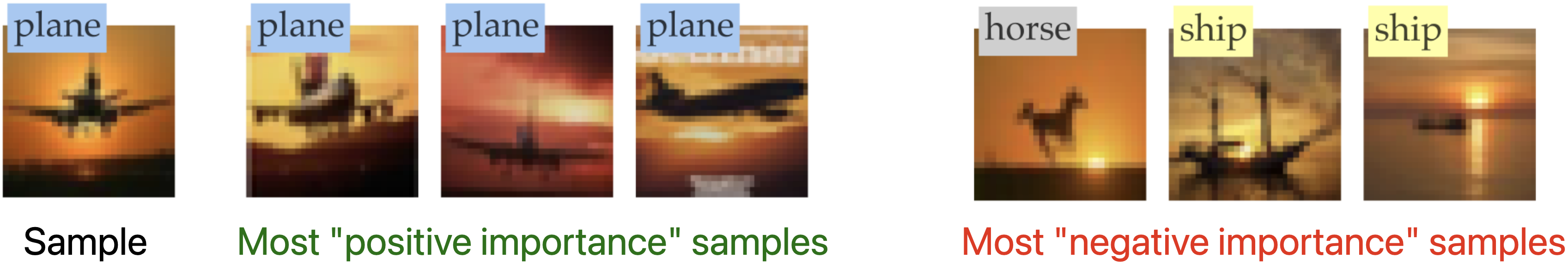
Analyzing these samples gives an obvious potential hypothesis for why the model mispredicted: the model associates sunsets with boats! With this hypothesis in hand, we can then test to see if it is indeed a mechanism that would explain the prediction (by first rigorously defining the hypothesis, then actually testing it; for example, we could “remove” the sunset from the image and inspect whether it changes the prediction).
What exactly do these importances mean? Exactly what “importance” means is dependent on the data attribution method of choice. In what follows, we briefly describe at a high level what these “importances” could mean in each category of data attribution; for a full overview of each method see Chapter 1 of the tutorial.
- Predictive data attribution: when the data attribution method is “linear” (cf. Chapter 3) in the choice of the training data, the “importance” for a given training sample is effect of including that sample in training on the prediction.
- Game theoretic: in the data Shapley setup, this importance could represent the “fair payoff” to each training datapoint, divided among the overall utility achieved by the model on the test point (e.g., negative loss).
- Corroborative: in this setting, the importance could represent the distance between each training sample and the test point. While this importance is model agnostic, it could still be useful for identifying potential patterns in the training data.
In the wild. There are many works on using data attribution methods to identify potential explanations for model behavior. These methods typically go beyond simply inspecting the top “importance” samples to look at principle components in data space or other more complicated schemes [Koh Liang 2017; Yeh et al. 2018; Ghorbani Zou 2019; Pruthi et al. 2020; Basu et al. 2020; Tang et al. 2021; Ilyas et al. 2022; Shah et al. 2022; Karlaš et al. 2022; Grosse et al. 2023; Rosenfeld Risteski 2023; Konz et al. 2023; Marion et al. 2023; Singla et al. 2023; Zheng et al 2024].
Three predictive data attribution applications
More alike than different
We now detail three separate applications—dataset selection, machine unlearning, and data poisoning—under a common, predictive data attribution framework. In this section, we start by describing the setting used across all the applications. We then detail the common framework, before discussing each individual application separately.
Setting
Let’s begin by recapping setup from Part II and Part III that recur throughout the applications below. We consider a universe of possible training data $U$, a learning algorithm $\theta$ mapping training subset to model parameters, and a model output function $f$ mapping an example $z$ and model parameters $\theta(S)$ to a corresponding output $f(z; \beta)$ (for example, $f$ could output loss/logits on the sample). Given a sample $z$ of interest, we assume access to a (predictive) data attribution estimate of the model output, \(\hat{f}_z(S) \approx f(z; \theta(S))),\) which estimates the predictions of a model trained on $S$. How can we apply such a primitive?
A simple formula for applying predictive data attribution
While these applications constitute entirely different machine learning tasks in practice, we show that each is solvable with a single straightforward formula.
This formula proceeds in two steps for a given task:
- Rewrite the problem as a prediction or optimization problem in terms of model outputs (i.e., in terms of $f(z; \theta(S))$).
- Plug in a predictive data attribution method to approximate the model outputs from the first step (i.e., use the estimates $\hat{f}_z(S) \approx f(z; \theta(S))$ in place of model outputs), then solve the resulting (much simpler) optimization problem.
Dataset selection
In dataset selection, the goal is to select the best subset for model training out of all the available data. This may seem like a strange goal: why not train on all the training data? It turns out that in many realistic settings, much of the available training data hurts downstream performance. For example, in language and vision settings we often train on internet data, which often contains spam, malformed text, and incorrect information. In practice, removing bad data (and keeping good data) from internet scrapes before training can greatly improve model performance.
However, determining which data is “the best” is tricky. This is where data attribution comes in: data attribution methods help identify which training data helps (and which data hurts) model training.
Step 1: Dataset selection in terms of model outputs. Dataset selection can be phrased as an optimization problem where the goal is to choose the training data that minimizes model loss. In this view, we aim to select the (predetermined, size $m$) subset of data $S^* \subset U$ that most reduces target loss (loss on a given target distribution $D_{targ}$; e.g., in a language setting this could be a suite of common LM benchmarks) when trained on, or the set
\[S^* = \arg\min_{S\subset U, |S|=m} \mathbb{\hat{E}}_{z \sim D_{targ}} \left[ \ell(z; \theta(S))\right]\]However, optimizing over choice of training data is difficult. Usually we optimize over parameters–not training data choice. While we can maximize with respect to parameters via first order methods, there are no known (efficient) methods for directly optimizing over model performance with respect to the training data choice. In general, it is unclear how to calculate the best training subset without enumerating over every possible subset and checking for the best model.
Step 2: Plugging in data attribution. We cannot optimize through model training with respect to training data: the function mapping training data to target loss is too difficult to optimize directly. To circumvent this problem, we operate in two stages: (a) approximate this function using data attribution, then (b) optimize over the approximation (data attribution outputs tend to be straightforward to optimize over with respect to data).
To approximate the function, we use data attribution directly. We approximate the downstream loss on each sample as (taking our $\hat{f}$ from above as modeling the loss): \(\hat{f}_z(S) \approx \ell(z; \theta(S))\)
We then use this approximation to estimate the best possible training dataset selection by optimizing:
\[\hat{S}^* = \arg\min_{S\subset U, |S|=m} \mathbb{\hat{E}}_{z \sim D_{targ}} \left[ \hat{f}_z(S)\right].\]In practice, solving this optimization problem is generally straightforward as data attribution estimates tend to be simple (for example, a standard form is $\hat{f}_z$ as a linear function of the choice of training data, as in Chapter 3).
In the wild. A number of methods select datasets with data attribution, ranging from those using predictive data attribution [Wang et al. 2023; Engstrom et al. 2024; Xia et al. 2024; Jiao et al. 2024; Chhabra et al. 2024] to those using game theoretic attribution [Schoch et al. 2023; Wang et al. 2024].
Resources. Data selection and curation are emerging fields that have attracted a lot of recent interest! There are a number of dataset selection challenges (e.g., DataComp and DataComp-LM) as well as curated datasets like FineWeb and Dolma that continue to show how to improve machine learning models by improving data.
Machine unlearning
Machine unlearning is the task of removing the effect of training on a given “forget set” of training samples on model outputs. This problem is particularly relevant in model deployment scenarios, where providers must satisfy users who (often backed by privacy-first government regulations) want their personal information removed from models. For example, after accidentally uploading private information to a service, a user may want the company to remove their information from trained models.
An effective approach to machine unlearning would be to train a new model every time that a new forget set (i.e., an additional request to delete a training sample) comes in. However, in large-scale model settings it is generally intractable to retrain a model for each new forget sample. Machine unlearning methods provide an alternative to retraining. These methods aim to modify existing, trained models’ outputs to match those that would have arisen if the models had not seen “forget samples” at train time.
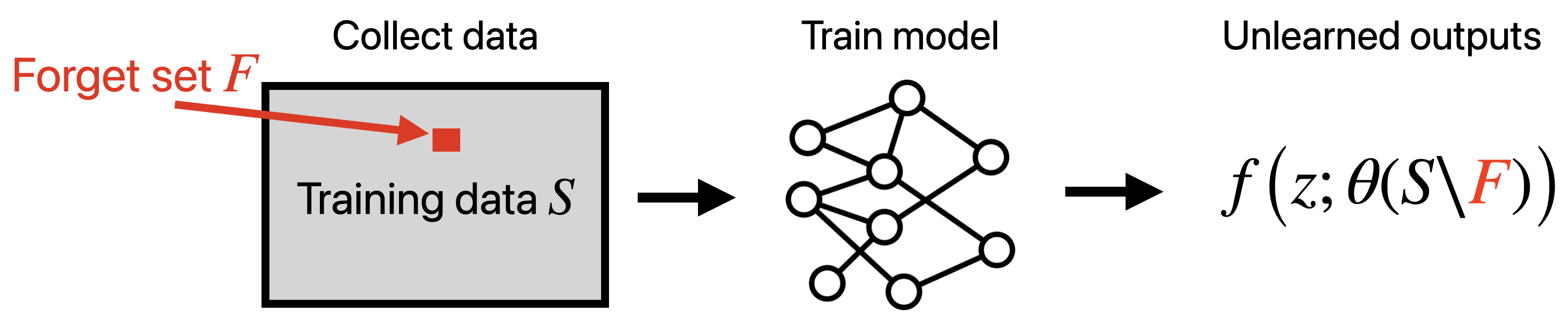
Step 1: Machine unlearning in terms of model outputs. Consider existing parameters $\theta$ fit to a training dataset $S$ and a model prediction function $f$ mapping sample and parameters to model predictions (e.g., logits in a classification setting). Given a “forget set” of training points $F \subset S$, the goal of unlearning is to estimate the predictions of a model trained without the forget set $F$ for arbitrary test samples $z$. This is exactly the problem of estimating the predictions: \(f(z, \theta(S \setminus F)).\)
Step 2: Plugging in data attribution. We can use data attribution methods to estimate these predictions. After all, given a test sample $z$, our data attribution method $\hat{f}_z$ yields estimates of how a model would predict on $z$ as a function of the training set. Therefore, our unlearning prediction estimate is just the data attribution estimate of how the model would predict without training on the forget set:
\[f(z; \theta(S \setminus F)) \approx \hat{f}_z(S \setminus F).\]In the wild. There are a number of methods for performing machine unlearning with data attribution-based approaches, and are often much more involved than the method outlined above due to real-world snags [Guo et al. 2020; Sekhari et al. 2021; Suriyakumar et al. 2022; Tanno et al. 2022; Warnaco et al. 2023; Pawelczyk et. al 2023]. The direct connection between predictive data attribution and machine unlearning was pointed out in an (upcoming) paper [Georgiev et al. 2024].
Resources. Benchmarks for evaluating machine unlearning are still under *active development. Recent popular benchmarks (across both supervised learning and generative modeling) include TOFU, MUSE, and ULiRa.
Data poisoning
In data poisoning attacks, there is an attacker that aims to hurt model behavior by modifying a small part of the training dataset. Such a threat model is a concern in many settings, as today’s model trainers collect data from sources ranging from the public internet (where anyone can post) to untrusted third parties like Amazon Mechanical Turk.

Depending on the exact manner in which the attacker aims to hurt model performance, this attack can be difficult to execute. How exactly should one modify training data to most hurt model performance? Data attribution methods provide one answer. (Note: understanding how to attack is useful for defending against poisoning as well!)
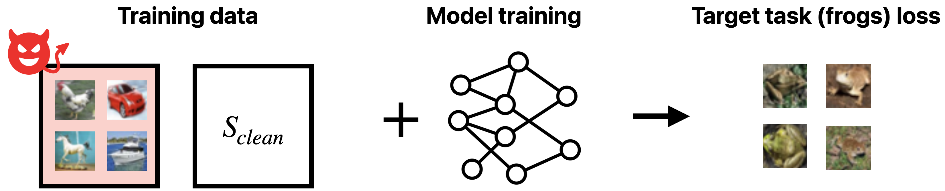
Step 1: Data poisoning in terms of model outputs. Consider a training set $S = S_{clean} \cup S_{adv}$ for which an adversary has complete control over the (small, fixed size) subset $S_{adv}$. The adversary knows that the defender will learn a model on the combined training dataset. The goal of the adversary is to construct a set of poisoned samples $S_{adv}$ that maximally hurts the performance of the trained model $\theta(S_{clean} \cup S_{adv})$ on a target set, $D_{targ}$. Here, $D_{targ}$ is a given task that we want to “poison”; for example, poisoning the “frog” CIFAR-10 class as below:
Viewed as an optimization problem, the adversary aims to solve maximize target loss after training: \(\underset{S_{adv}}{\operatorname{max}}\ \mathbb{E}_{z \sim D_{targ}} \left[\ell(z; S_{adv}\cup \theta(S_{clean})\right].\)
Step 2: Plugging in data attribution. This objective is hard to maximize directly, as it is difficult to optimize through the model training process with respect to input data. This is the same problem we had performing dataset selection above: model training is a complicated function. Instead, we can replace the model training process with a data attribution-based proxy. One can approximate the target loss after training on a given training dataset as: \(\mathbb{E}_{z \sim D_{targ}} \left[\hat{f}_z\left(S_{adv}\cup S_{clean}\right)\right] \approx{} \mathbb{E}_{z \sim D_{targ}} \left[\ell(z; \theta(S_{clean}\cup S_{adv})\right];\) then maximize this proxy in place of the original objective. The full optimization problem is then to maximize loss on the target:
\[\min_{S_{adv}} \mathbb{E}_{z \sim D_{targ}} \left[\hat{f}_z\left(S_{adv}\cup S_{clean}\right)\right].\]In the wild. There are a number of works poison that poison training data in a similar manner, though many of them do not explicitly use the data attribution framing [Biggio et al. 2012; Koh Liang 17; Xiao et al. 2018; Fang et al. 2020; Koh et al. 2022; Wu et al. 2023].
Wrapping up
Many of the applications that we’ve discussed here are still in their infancy, and exciting new applications of data attribution are continually arising. Broadly, we are excited about the general recipe discussed in this section—where one first writes down an optimization problem then plugs in data attribution in place of model outputs—as a versatile primitive for applying predictive data attribution.
The way forward for data attribution. Despite rapid progress in recent years, data attribution methods have not really found adoption in production settings. We think there are a couple reasons for this. First, data attribution methods are not well-known model debugging tools for practitioners [Nguyen et al. 2023]. Second, we think that even within academia, data attribution is often viewed only a descriptive tool for studying and understanding machine learning models. (We hope that this tutorial makes a convincing case that they can actually be useful tools for building and improving ML systems as well.) Finally, while methods are continually improving, existing data attribution methods are not still not accurate enough to be reliable in large-scale settings. Still, we do not think any of these challenges are fundamental, and in particular, we expect data attribution to become a standard part of the machine learning toolkit within the next 5-10 years.
This concludes our tutorial on (predictive) data attribution. We hope you’ve found some of the material useful! Please reach out to ml-data-tutorial@mit.edu with any comments or questions.