
III: Scaling to deep learning
In the previous chapter, we saw that in classical regimes, there are reliable methods for (a close statistical analog of) the predictive data attribution problem. In this section, we’re going to explore predictive data attribution in modern-large scale settings—it turns out that the landscape here is quite a bit more complex.
A first attempt: directly applying the influence function
Recall from Part II the leave-one-out problem:
\[LOO(j) = \left(\arg\min_\theta \sum_{i=1}^n \ell_i(\theta)\right) - \left(\arg\min_\theta \sum_{i\neq j} \ell_i(\theta)\right),\]and its corresponding “influence function estimate”
\[\widehat{LOO}_{\text{IF}}(j) = \left(\sum_{i=1}^n \nabla^2 \ell_i(\theta)\right)^{-1} \cdot \nabla \ell_j(\theta).\]We found that this estimator was remarkably predictive and even come with provable guarantees when the loss functions $\ell_i(\cdot)$ are strongly convex. In light of this, a natural first question to ask is: can we simply apply the exact same estimator in the context of deep learning.
On one hand, essentially all the assumptions we made in Part II are violated in deep learning—for example, neural networks are non-convex problems; we typically do not train models to convergence; and the parameters themselves are not identifiable due to randomness in model initialization and training. These violations pose both technical problems (e.g., how do we invert a possibly non-invertible Hessian?) as well as conceptual ones (e.g., if the global solution is not unique, what is the influence function even computing [BNL+22]?).
On the other hand, many of the most successful techniques in deep learning use intuition from classical problems, and work in practice even when major assumptions are violated (see, e.g., the use of momentum in convex optimization). Inspired by success stories like these, we might want to try ignoring these issues for now, and applying the same Taylor-based approximations from Part II (e.g., the influence function estimate based on the infinitesimal jackknife)It turns out that, assumption violations aside, even just computing the IF estimate is highly non-trivial. This is, in part, due to high-dimensionality and non-invertibility of the Hessian. We’ll sweep these issues under the rug for now, and just assume we are able to compute the relevant quantities. .
A pioneering paper by Koh and Liang [KL17] takes exactly this approach. They develop clever techniques to compute influence function (IF) estimates (adapting the estimator above to estimate changes in model predictions, rather than model parameters) that accurately predict how model behavior changes with choice of training data weights in smaller settings (small MLPs, CNNs, and for linear models trained on the last layer representations of an Inception-v3 model). In particular, the leave-one-out estimates they get correlate remarkably well with true leave-one-out effects (computed by re-training the model):
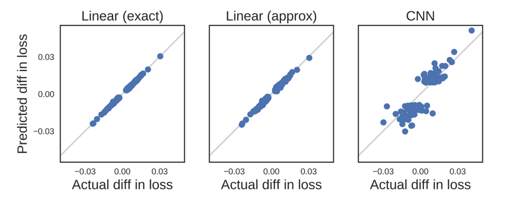
(Figure 2 from [KL17]). Right shows fidelity of IF approximation for a small CNN trained on MNIST
In an accompanying Jupyter notebook, we present a simple (~200 lines of code) implementation of this method, highlighting the main technical ideas from [KL17].
[KL17] and subsequent works leverage the influence function for a variety of applications, such as identifying mislabeled or poisoned data, debugging model behavior, or cleaning datasets, suggesting their potential utility. Often, the attributions appear to pass heuristic “sanity checks” like visual similarity—the most “influential” examples bare some resemblance to the target example.
However, other subsequent works have found that under closer scrutiny, variants of these approaches are unreliable for DNNs:
- [BPF’21] find that the IF estimates are extremely fragile, depending on hyper-parameters (regularization), and things generally get worse with wider or deeper networks:
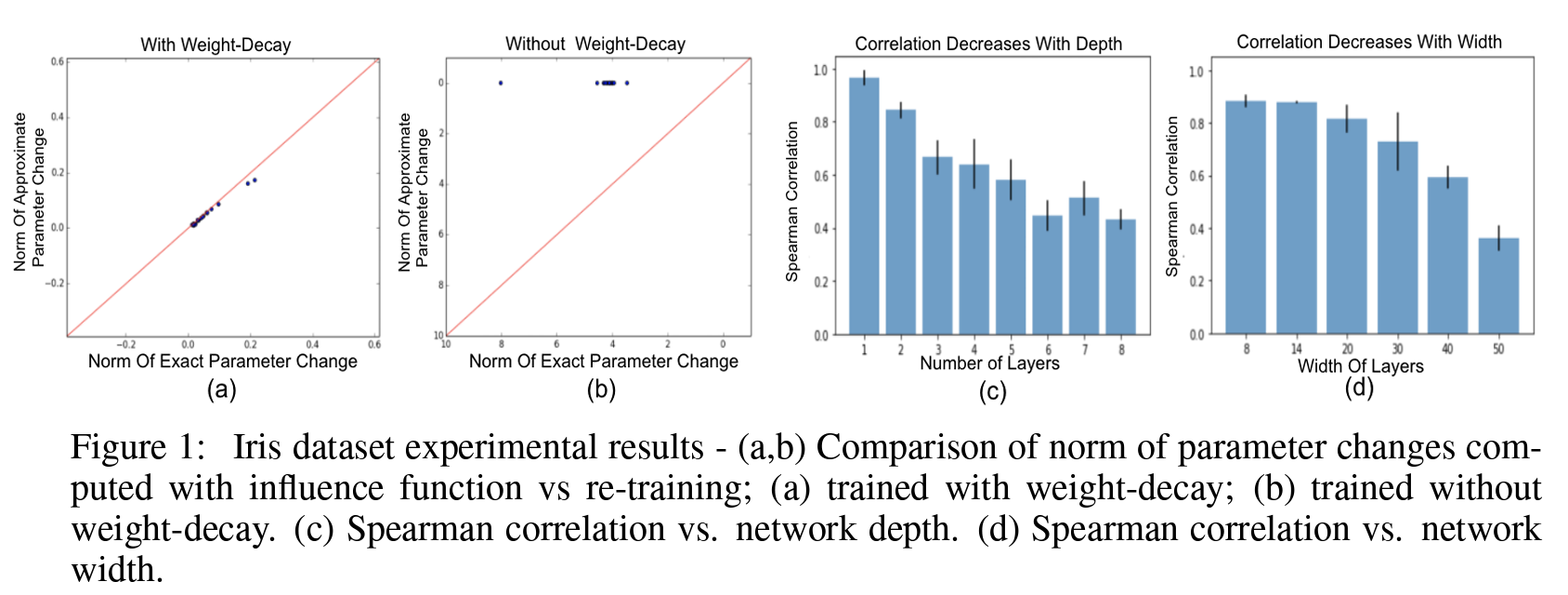
Reproduced from Basu et al.
- [HL’22] find that existing methods fail at even simple sanity checks: if you compute the influence scores on dataset A and B (e.g., CIFAR-10 and MNIST) to a target example from A, often the most influential examples according to existing attributions are from B rather than A!
- If we think a bit more carefully, it’s not even clear what these influence estimates are even predicting, as so many assumptions from the convex setting are violated. Bae et al. [BNL+22] carefully analyze these issues, and suggest that in the context of deep neural networks, influence functions actually estimate a different quantity entirely than $LOO$.
Some of these inconsistencies are not easily detectable based on manual inspection of the estimated attribution scores. These findings highlight that we cannot use heuristics like human inspection or visual similarity to judge the quality of predictive attributions. After all, the reason we are trying to attribute model behavior to data in the first place is precisely because models often behave in strange ways!
What do we do next? On the one hand, we could try somehow correcting the influence function estimates—perhaps there’s a better way to apply it to ML contexts. Or perhaps the approach is doomed and we need to use other ML-specific techniques to estimate LOO. These are all reasonable approaches that have been explored in the literature and we’ll actually talk about some of them later, but right now we have a more fundamental problem.
It’s clear that what we have right now isn’t reliable—we have failed sanity checks and theoretical analysis to show this. But in coming up with new methods, how will we know when we’re making progress?
Quantifying predictive data attribution
Before we can blaze ahead designing better methods for predictive data attribution, we need a good way of knowing when we’re actually making progress. There are many things we could do here: we could re-use some of the sanity checks from above (as in HL20); we could try to measure parameter-space differences (as in BPF20); or we could look at leave-one-out scores (as in [KL17; BNL+22]). Recall from Part I, however, that our goal at the end of the day is to predict how training data influences final model behavior.
Inspired by this goal, we formalize an idea that’s been floating around in the literature on training data attribution: the most direct thing we can do to evaluate a predictive data attribution metric is measure its prediction error relative to model re-training. The result is what we call the Linear Datamodeling Score [IPE+’22; PGI+23] (LDS). First, recall from Part I the definition of a predictive data attribution method:
Definition [Predictive data attribution method]. Consider a universe of data $\,\mathcal{U}$, a training algorithm $\smash{\theta(\cdot): 2^\mathcal{U} \to \mathcal{M}}$ mapping training sets $S$ to machine learning models, and a measurement function $\ell: \mathcal{M} \to \mathbb{R}^k$ recording some property of a machine learning model (e.g., its loss on a set of test examples). A predictive data attribution is a function $\hat{f}: 2^\mathcal{U} \to \mathbb{R}^k$ that directly approximates the result of training a model and evaluating $\ell$, i.e., $\hat{f}(S) \approx \ell(\theta(S))$ for all $S \subset \mathcal{U}$.
Note that the definition above is given in terms of all subsets $S \subset \mathcal{U}$. While this is indeed the end goal, in practice predictive data methods aren’t quite there yet—so instead, we’re going to measure the average performance of data attribution methods across a distribution over training sets $S$:
We’ll often be interested in the “per-example” LDS, which is when the measurement function $\ell$ measures the loss of a model on a specific test example $z$. We generally denote the resulting example-specific data attribution as $\smash{\hat{f}(z; S)}$.
Let’s digest this definition with some code. First, we create subsets $\lbrace S_1,\ldots,S_m\rbrace $:
# 1. create 10 random subsets of the training set
# (each containing a half of the universe of 50,000 points)
import numpy as np
np.random.seed(42)  # fix random seed for reproducibility

train_set_subsets = []
for i in range(10):
    subset = np.random.choice(range(50_000), 25_000, replace=False)
    train_set_subsets.append(subset)
Then, to obtain the true model output $\ell(\theta(S_j))$, we need to first train a model on each subset $S_j$, and then evaluate it on a target example $z$:
# 2. train a model on each subset and record
# its output on a target example of choice
from utils import train_on_subset, record_output, get_loader

val_loader = get_loader(split="val")
target_example = val_loader.dataset[0]

outputs_per_subset = []
for subset in train_set_subsets:
    model = train_on_subset(subset)
    out = record_output(model, target_example)
    outputs_per_subset.append(out)
Finally, we use our data attribution method of choice to get predicted model output $\smash{\hat{f}(z, S_j)}$ for each subset $S_j$, and report the rank correlation between the two arrays:
# 3. evaluate the rank-correlation between the true model
# outputs and the predictions from our attribution method
from scipy.stats import spearmanr

method = FavTDAMethod()
method.fit(model, ...) # pre-compute attribution scores
predictions_per_subset = [method.get_predicted_output(subset, target_example) for subset in train_set_subsets]

LDS = spearmanr(outputs_per_subset, predictions_per_subset)
print(f'LDS: {LDS.correlation:.3f} (p value {LDS.pvalue:.6f})')
For convenience, we have put together the above snippets in this Jupyter notebook.
With this formalization, our goal is to design data attribution methods $\hat{f}$ that achieve a high LDS.In practice, evaluating LDS requires training many models (~100) on different training datasets. Though expensive, note that this cost is upfront; it is independent of the attribution method, so we can train these models and record their outputs in advance, and then evaluate any subsequently attributions. The LDS has been used recently to evaluate credibility of attributions across various domains [PGI+23; GVS+23; DZM23; ZPD+23; BLLG24; DLZM24].
Revisiting our initial estimator
Now that we have a clearer picture of what to evaluate, we can revisit and evaluate some of the initially proposed estimators. Below, we evaluate the influence function estimator [KL17] in the setting of ResNet-9 classifiers trained on CIFAR-10:
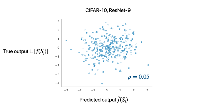
We observe that the LDS is very low. In other words, this means that the influence function on its own cannot reliably predict what happens to predictions when we train models on random subsets of a larger training pool. (Note that this doesn’t preclude this estimator from being useful—LDS only evaluates methods in their capacity as predictive data attribution techniques.)
Is data attribution even possible for DNNs? Direct estimation
Note that the influence function estimator we derived in Part II is linear in that we can decompose it into the following form:
\[\hat{f}(S) = \sum\limits_{i\in S} \tau_i\]But large model training (particularly for non-convex models like neural networks) is an incredibly complex process—is it possible that we just can’t predict with a simple linear model?
To understand this better, we’re going to directly try to learn the data-to-model-output mapping. That is, we treat our task as a statistical learning problem of $S’\mapsto \ell(\theta(S’))$ and approach as follows:
- Repeatedly train models $\theta(S_i)$ on random samples $S_i \subset S$, and collect the corresponding model outputs $\lbrace \ell(\theta(S_i))\rbrace $.
-
Now we have a simple regression problem from $2^{\vert S\vert}$ to $\mathbb{R}$: $\lbrace (S_i, f(x,S_i))\rbrace $. While we can consider any family of functions, [IPE+22] finds that perhaps the simplest instantiation of using linear models suffices, i.e., we can solve:
\[\min_{\tau \in \mathbb{R}^n} \frac{1}{m} \sum_{i=1}^m (\tau^\top \mathbb{1}_{S_i} - \ell(\theta(S_i)))^2 + \lambda \cdot \text{reg}(\tau)\]where $\mathbb{1}_{S_i} \in \lbrace 0,1\rbrace^N$ is the indicator vector encoding $S_i$ and $\text{reg}$ is a regularization term (e.g., $\ell_1$ norm to promote sparsity).
Interestingly, the resulting estimator ends up being very related to (i.e., a slight refinement of) previously-suggested data attribution methods, both predictive and game-theoretic [GZ19, FZ20; IPE+’22; LZL+’22]!
Note that we estimate such a linear model for each choice of target input $z$. Here, we overload the notation so that $\tau(x)$ is the estimated datamodel for $x$ computed using the attribution method $\tau$.
The resulting datamodels achieve very high LDS (and generally perform better with more samples):
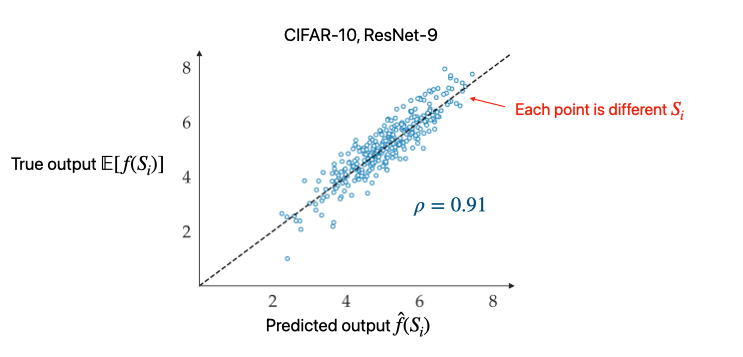
Before we go further, this establishes that our goal of predictive attribution is actually attainable in modern settings! This is a crucial point: a priori, it’s not clear we can model the complicated function $f$ with any fidelity.
Now, in some sense this direct approach should also give optimal estimates with infinite compute. The downside is that this procedure is often prohibitively expensive, as this requires many model re-trainings (e.g., one needs ~10,000 models for the CIFAR-10 dataset to get a decent LDS).
Predictive data attribution in modern settings
We saw that it is possible to find predictive linear models even in the DNN setting. Influence functions worked great for classical problems like logistic regression—so what changed?
There are a number of changes that complicate things for us, including some we alluded to earlier:
- Non-convexity: The Hessian of a DNN is in general no longer going to be positive definite, so its inverse will not be well defined. One can try accounting for this by adding regularization or other tricks, but it’s not clear if these post-hoc fixes are the right approach.
- Randomness: DNNs are stochastic in nature; re-training a model with a different random seed will lead to a completely different set of parameters. This means that we have to more careful about reasoning in parameter space directly.
- Non-convergence: We typically do not train DNNs to convergence (even locally), so it is questionable to rely on convergence assumptions that were previously used in deriving the IF estimates.
- Large-scale/high-dimensionality: Due to the high dimensionality of modern overparameterized models, exact second-order computations are infeasible (i.e., it’s prohibitevly expensive to compute the exact Hessian, even if our objective were convex).
Various methods have been proposed to deal with some of the problems above. Next, we’ll give a broad overview of the main approaches.
A birds-eye view of modern predictive data attribution
Broadly, there are a few lines of approach that people have come up with. Namely:
- Better IF/Hessian approximations
- Approximating training dynamics directly (“unrolling”)
- Surrogate models
While the direct estimator earlier treated the DNN as a blackbox, each of these approaches try to approximate the blackbox more accurately based on different assumptions about properties of DNN training. We’ll now give intuition for each of these approaches, focusing on one or two successful methods for each approach.
I. Approach: Better IF approximations. Some methods directly tackle the original IF approximation. There are many different variations on this theme, but two key trends that have emerged from recent works [TBG+21; GBA+23; CAB+24] are:
-
Intead of approximating the true Hessian directly, using the “Gauss-Newton Hessian” (GNH) approximation, given by:
\[G := \mathbb{E}[J^T H_{\hat{y}} J],\]where $J = d\hat{y}/d\theta$ is the parameter-output Jacobian and $H_{\hat{y}}$ is the Hessian of the training loss w.r.t. to the network’s outputs. This can be interpreted as computing the Hessian of the linearized network (that is, replacing the original model with its linear approximation in parameter space). This change addresses non-convexity, as this new Hessian is guaranteed to be positive-semidefinite.
-
Further structural approximations that make above more tractable: For example, the K-FAC [Martens Grosse ’15] based estimation assumes that i) the gradients across different layers; and further ii) the activations and the inputs to linear layers are independent. i) introduces a “block-diagonal” structure that allows one to compute the inverse of the Hessian by inverting each block separately, while ii) allows one to express the gradients of linear layer weights as a kronecker product of two much smaller vectors. These approximations signifcantly speed up the inverse-Hessian-vector products needed to compute the IF estimates. Furthermore, some type of spectral regularization is also employed (approximating each block by its top eigenspace).
There is a rich line of work on Hessian-free optimization that provides some intuition for why the above approximations are reasoable—and perhaps even desirable–compared to the original exact Hessian [Martens ’14].
In summary, these methods tackle the challenges of non-convex settings by finding better and more efficient structural approximations to the Hessian, the key object in the IF estimate.
For an implementation of this type of approach, check out the Kronfluence repository.
II. Approach: Approximating training dynamics. The methods thus far only look at the final trained model, but doesn’t account for the trajectory of how we got there. Given the unsuitability of the IF approximation and our understanding of the importance of implicit biases, it makes sense to look at the entire trajectory. At a high level, “unrolling” based methods try to “trace” the training dynamics across multiple checkpoints to more accurately predict the counterfactual trajectory resulting from a different training set.
To begin, recall that the IF is computing this derivative (see Chapter 2 for details):
\[\frac{d\theta^{(T)}}{ {dw_j}_{\phantom{t}}},\]the infinitesimal effect of up-weighting example $j$ by $\epsilon$ on final parameters $\theta^{(T)}$. But this required a lot of assumptions on $\theta^{(T)}$ and the loss function. So instead, we’re going to try to compute the above quantity by exactly tracing the entire trajectory of parameters $\lbrace \theta^{(t)}\rbrace _{t=1,…,T}$.
Let’s look at an example of analyzing full-batch gradient descent, where we perform the updates:
\[\theta^{(t+1)} = \theta^{(t)} - \eta_t \cdot \sum_{i=1}^n \nabla \ell_i(\theta^{(t)})\]($\eta_t$ is the learning rate at step $t$)
-
First, we start by looking at something simpler, the effect of up-weighting the example $j$ by $\epsilon$ only at iteration $t$ on final model parameters $\theta_T$ (denoted by the LHS below):
\[\frac{d\theta^{(T)}}{dw_j^{(t)}} := \frac{d\theta^{(T)}}{d\theta^{(T-1)}}\cdots \frac{d\theta^{(t+2)}}{d\theta^{(t+1)}} \cdot \frac{d\theta^{(t)}}{dw_j^{(t)}}\]where the RHS follows simply via the chain rule from calculus.
Now, given the gradient update rule, we can compute the quantities in the above expression in closed form. For the rightmost term:
\[\frac{d\theta^{(t)}}{dw_j^{(t)}} =\eta_t \nabla_\theta \ell(z_j, \theta^{(t)})\]For all intermediate terms, we can derive by simply differentiating the gradient update rule w.r.t. $\theta^{(t)}$:
\[\frac{d\theta^{(t+1)}}{d\theta^{(t)}} = (I - \eta_{t-1} H_{t-1})\]where $H_t$ is the Hessian at time step $t$.
Substituting these back into original expression, we have:
\[\frac{d\theta^{(T)}}{dw_j^{(t)}} = (I - \eta_{T-1} H_{T-1}) \cdots (I - \eta_{t} H_t) \cdot \eta_t \nabla_\theta \ell(z_j, \theta^{(t)})\]where $H_t$ is the Hessian at time step $t$.
-
Next, by summing over the above expression for all iterations $t$, we can the total effect of the entire training process w.r.t. $\epsilon$:
\[\frac{d\theta_T}{dw_j} = \sum\limits_{t=0}^T \frac{d\theta_T}{dw_j^{(t)}}\]which is just due to the total derivative rule.
At the end, this gives an exact closed form expression! However, computing it (naively) would require storing checkpoints at every iteration and storing many Hessian matrices (or at the least, computing many Hessian-vector products), so it is not really tractable to compute. So different methods aim at approximating the above quantity:
A first-order approximation: One approximation is a popular method called TracIn [PLSK20], which ignores all the second-order effects (the $\frac{d\theta^{(t-1)}}{d\theta^{(t)}}$ terms). This simplification removes all the Hessians and requires you to keep only track of the gradients. Then, the overall influence on final model parameters can be approximated as the sum:
\[\sum_{t=0}^T \nabla_\theta\ell(x_j,\theta^{(t)})\]However, this introduces significant bias into the estimates; indeed, if we consider just least-squares regression, we can find that TracIn already gives a very skewed estimate (an exercise for the reader—remember from Part II that we have a closed form for leave-one-out scores here!).
A better approximation. A more recent method SOURCE [BLLG24] does a much more faithful approximation. At a high-level, the method breaks the time steps into a few segments, and assumes that the Hessian is approximately constant within each segment. This allows you to get by only storing a few intermediate checkpoints. In the end, this approximation yields very good estimates (e.g., outperforms other approaches on recent LDS benchmarks).
Other works such has Simfluence [GWP+23] take a more modeling-based approach and model the entire trajectory with a Markov process.
To summarize, the main idea behind these methods address non-convexity by more directly modeling the sequential training process of DNNs. These methods also implicitly deal with randomness by averaging over multiple checkpoints. However, keeping track of all the information about optimization (gradients, Hessians) gets quickly unwieldy, so different methods leverage various approximations.
III. Approach: Surrogate models. For simple models (such as the linear models we saw in Part II, or other simple classes like k-NN), we actually do know how to do predictive data attribution. To that end, the idea behind this final approach is to find a proxy or surrogate model that approximates the neural network, and compute data attributions on the proxy model.
For example, a line of work uses k-NN classifiers as a proxy for the original model [JDW+19]. Applying influence functions to the last layer embeddings (used in a few works, e.g., KL17) can also be viewed as using a linear proxy model on those representations.
Here, we briefly describe one successful approach called TRAK [PGI+23]. At a high level, TRAK reduces to a generalized linear model (GLM)—e.g., logistic regression—and applies the influence function approximation to the GLM. We can break this down into three steps:
-
Linearize the original DNN (represented as a function $h$):
\(h(x,\theta) \approx h(x,\theta^\star) + \nabla_\theta h(x;\theta^\star)\cdot (\theta-\theta^\star)\).
This allows us to reason instead about a linear model whose features are given by $\phi(x) := \nabla_\theta h(x;\theta^\star)$. The motivation for such can approximation is loosely based on recent works on the eNTK approximation [L21; WHS22; MWY+23; VAB+23].
- We can further reduce this to a more tractable low-dimensional model by randomly projecting the features: $P^T \phi(x) \mapsto \tilde{\phi}(x)$ using some projection matrix $P$. Intuitively, as long as we approximately preserve the geometry, the proxy model won’t change too much from the true linearized model (see, e.g., [LPJ+22; AZP24] for some intuition).
- We can then apply the standard IF approximation (from Part II) to this corresponding linear model to perform predictive data attribution.
- Lastly, we can ensemble the earlier steps over multiple checkpoints and projections to reduce variance.
Despite the number of approximations involved, the resulting estimates are surprisingly good (in terms of LDS), and allow us to approximate direct estimators while being orders of magnitude more efficient.It turns out that one can also view TRAK as an (efficient) approximation of the Gauss-Newton Hessian; in particular, one can view TRAK as an “agnostic” approximation leveraging randomness rather than the structural approximations made by EK-FAC and related methods. As shown in the plots below, these have different trade-offs.
For a fast and flexible implementation of TRAK, check out the code on GitHub. For this tutorial, we also provide a simple & hackable implemenation in this Jupyter notebook.
Evaluating the landscape
To get a sense of how these different methods perform on different target tasks, we evaluate a representative set of these methods (and simpler baselines) across three settings: ResNet-9 models trained on CIFAR-10, BERT models fine-tuned on QNLI, and GPT-2 models fine-tuned on WikiText. On the y-axis, we evaluate the effectiveness of the attribution method using the LDS, and on the x-axis we quantify its efficiency based on GPU runtime. Recent unrolling-based method SOURCE, is currently missing from the figure above; see their paper for comparisons.
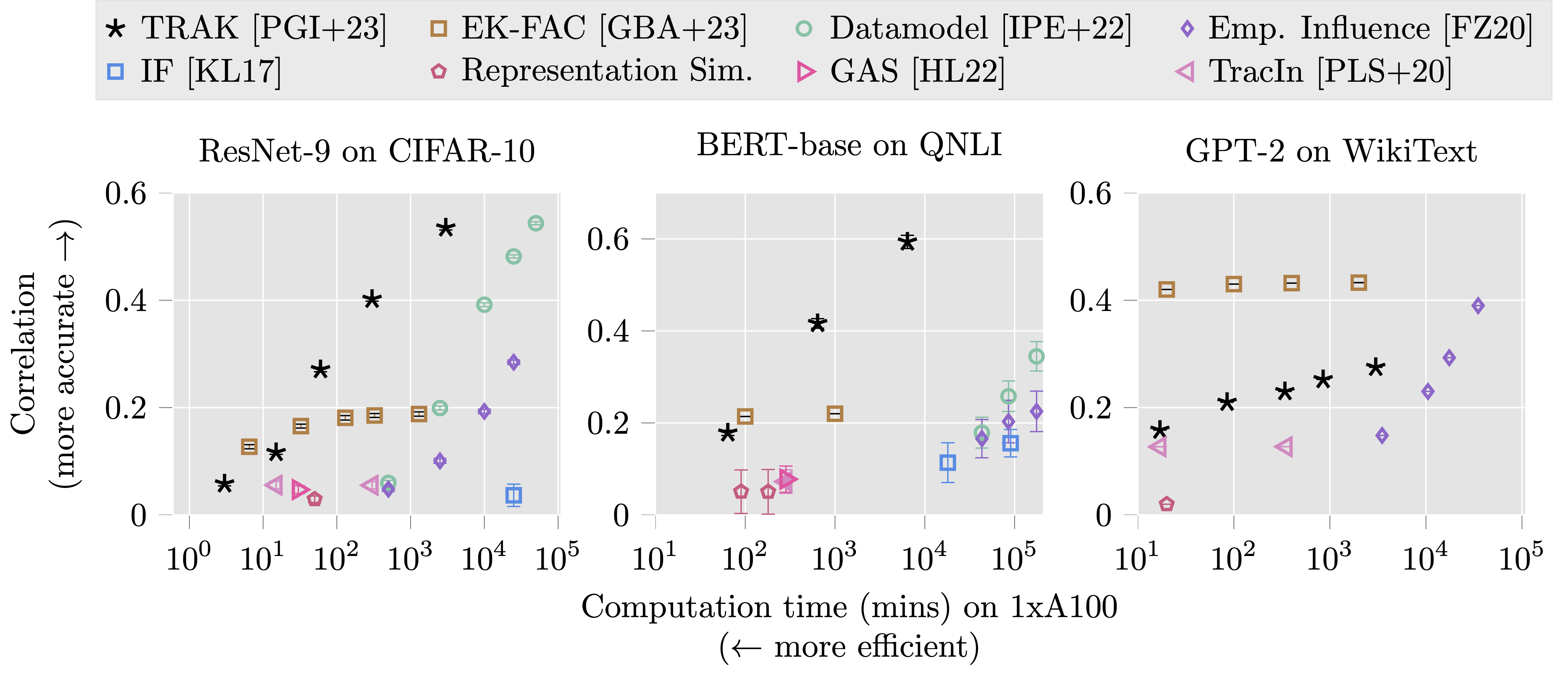
We observe the following trends:
- Commonly used baselines (original adaptation of influence functions to DL, representation similarity, and TracIn) not very predictive, regardless of compute.
- Direct estimators (e.g., regression-based datamodels) perform best with enough compute.
- Recent efficient methods (e.g., TRAK, EK-FAC) manage to approach the performance of direct estimators in some cases.
- The best method (in terms of LDS vs time trade-offs) depends on the target task: e.g., TRAK is better on vision, EK-FAC better for language modeling (we suspect this is due to the difference in assumptions used by TRAK vs EK-FAC, and differences in structural properties CNNs and Transformers).
Overall, we do have fast, predictive, and reliable methods that seem to adapt well to different modalities!
Takeaways & (lots of) future work
We covered a lot of ground in this chapter, so let’s briefly recap the main takeaways:
- Evaluate countefactuals: If your goal is predictive attribution, you have to evaluate counterfactuals, using a metric like LDS. Practically, using the LDS can be a good way of choosing the best method for your given application (e.g., as different methods have higher LDS on different domains).
- Use good attribution methods: Many popualr baselines are not predictive, but some recent methods are realiably predictive.
- Choose method appropriate to modality: Beyond the original settings in which these methods were developed, newer techniques now adapt them pretty reliably across different modalities (e.g., language modeling [PGI+23; GBA+23], diffusion, etc.) Nice thing is that latest methods are pretty general and adapt readily to different settings out-of-the-box.
- Sanity check attribution method in simpler settings. Often, analyzing whether your new attribution method works in a simpler setting like a linear model can help us rule out some approaches easily. We did not go into more detail here, but this rules out some popular approaches like representation or gradient similarity.
While the field has matured a lot over the past several years, there’s still many interesting open problems. We end with some ideas for future research on predictive data attribution:
- More predictive methods: While we have reasonably predictive methods, they are far from what “oracle” estimates such as the direct approach yields. Can we improve on above approaches or use new ideas to get even better estimates? For example, are there better proxy models for DNNs? (Conversely, can we use our understanding of attribution methods to better understand the properties of DNNs?)
- Understanding beyond linearity: Most existing attribution methods use linearity (and they are surprisingly effective), but can we go beyond linear? Simple toy models suggest that modeling data interactions linearly cannot provide the full picture, so we must look for new methods that incorporate non-linearity (see, e.g, [WYZ+24] for insights along this line).
- “Single model counterfactual”: For most of this tutorial, we focused on attributing the average output of models (across re-training with different random seeds). But often in practice, we have a particular model we care about (e.g., GPT-4-Turbo-April03). How do we adapt methods and evaluations to such settings, where we only really get to observe a “single trajectory”?
- Multiple training stages: Modern models are trained via multiple stages (e.g., LLMs go through pre-training, then supervised finetuning and RLHF). Can we find methods that can flexibly deal with such scenarios? Recent methods provide some ideas.
- More efficient evaluation: To even know whether an attribution is working at all requires some type of counterfactual re-training, which quickly gets expensive. Can we find more efficient proxies to gauge whether attributions are predictive?
Now that we have saw that it’s possible to attribute predictions back to training data using modern tools, in the next section, we look at some of the exciting applications enabled by the primitive of predictive data attribution.
Some links and resources
Below is an incomplete list of resources that talk more about applying data attribution to modern settings:
Applying & studying convex data attribution at scale:
- Pang Wei Koh, Percy Liang. Understanding Black-box Predictions via Influence Functions (2017)
- Juhan Bae, Nathan Ng, Alston Lo, Marzyeh Ghassemi, Roger Grosse. If Influence Functions are the Answer, Then What is the Question? (2022)
- Samyadeep Basu, Philip Pope, Soheil Feizi. Influence Functions in Deep Learning Are Fragile (2020)
Inefficient-but-accurate methods:
- Vitaly Feldman, Chiyuan Zhang. What Neural Networks Memorize and Why: Discovering the Long Tail via Influence Estimation (2020)
- Andrew Ilyas, Sung Min Park, Logan Engstrom, Guillaume Leclerc, Aleksander Madry. Datamodels: Predicting Predictions from Data (2022)
- Jinkun Lin, Anqi Zhang, Mathias Lecuyer, Jinyang Li, Aurojit Panda, Siddhartha Sen Measuring the Effect of Training Data on Deep Learning Predictions via Randomized Experiments (2022)
State-of-the-art methods:
- Sung Min Park, Kristian Georgiev, Andrew Ilyas, Guillaume Leclerc, Aleksander Madry. TRAK: Attributing Model Behavior at Scale (2023)
- Juhan Bae, Wu Lin, Jonathan Lorraine, Roger Grosse. Training Data Attribution via Approximate Unrolled Differentiation (2024)